One of the most important skills we learn as physicists is how to approximate. The best physicists like Fermi or Feynman could turn this into a real art. Fermi for instance would tackle a question such as:
How many piano tuners are there in Chicago?
What’s your guess? Such problems became to be known as Fermi problems. By multiplying reasonable estimates (number of people in Chicago, number of people per house, percentage of households having a piano, how many times a year a piano needs tuning, how many pianos can a piano-tuner tune on a working day, etc.), one arrives at an estimate which, often, is surprisingly accurate. There is some statistics involved in the stability of such a procedure, that we will not go into today. Suffice to say that one of the most important and intriguing open questions ever posed to mankind relies on such an estimation (where is everybody? see the Drake equation).
Another useful approximation which every physicist uses is the linear approximation. This replaces an exact but awkward expression into an approximate but useful result. For instance, we have seen in the lecture on the double-slit experiment how the path difference reads straight from Pythagoras:
$$\begin{align}\Delta l&=l_2-l_1\\
&=\sqrt{(x+d/2)^2+L^2}-\sqrt{(x-d/2)^2+L^2}\tag{1}\label{eq:1}\\
&={L}\left(\sqrt{1+\left[\frac{x+d/2}{L}\right]^2}-\sqrt{1+\left[\frac{x-d/2}{L}\right]^2}\right)\\
&=\frac{xd}{L}\tag{2}\label{eq:2}\end{align}$$
and how this brings us to a useful formula—which we can keep in our collection of important results to remember—between the position of the $n$th bright fringe, at $x$, when light with wavelength $\lambda$ is projected on a screen a distance $L$ apart through a double slit of width $d$:
$$x=n\frac{\lambda L}{d}$$
The 2nd line, eq. (), is the exact result. The last line, eq. (), is the approximation when $L\gg x+d$. This is achieved by using so-called Taylor expansion, or Taylor series. Namely, we have used here the fact that:
$$\sqrt{1+\epsilon}\approx 1+\epsilon/2\tag{3}\label{eq:3}$$
which is a good approximation when $\epsilon\approx 0$. This is shown graphically below.
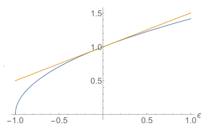
The blue line is ${\sqrt{1+\epsilon}}$ and the orange one is $1+\epsilon/2$. We have replaced a curvy shape by a line!
You can see how we approximate a complicated nonlinear function (here a square root) by a linear function. For instance, it is easy to compute that $\sqrt{1.012}$ is close to 1.006 (the real result is 1.00598, an error of less than 0.002%). It works fairly well even when $\epsilon$ is not that small. This is the percentage of relative error made:
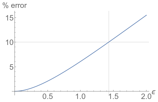
and for a qualitative understanding, 10% is acceptable. So you can happily estimate $\sqrt{1.75}$ as 1.375 (by mental calculation, we’d go first with 1.35 (1+0.7/2) and the time to say that, you could add the 0.05/2=0.025 but as this is an overestimation, as shown on the first graph, it’d be wise to stop there anyway. The real result is 1.32288, an error of about 2%).
An engineer, or a computer, would want to keep the exact result. A physicist would typically look for as much simplifications as possible (but not more). Actually, so great is the temptation that we even simplify very simple things that would not seem to require it, such as $(1+x)^2\approx 1+2x$. Here it’s from the binomial theorem. But for the general case, where does this come from anyway? At the first order, simply from the derivative, which is defined as:
$$f'(x)=\lim_{\epsilon\rightarrow0}\frac{f(x+\epsilon)-f(x)}{\epsilon}$$
That’s the definition of a Mathematician. For us, it becomes:
$$f'(x)\approx\frac{f(x+\epsilon)-f(x)}{\epsilon}$$
The limit means that it becomes exact when $\epsilon$ is vanishing. For any finite value, this is only an approximation (a better one the smaller the $\epsilon$, but an approximation nonetheless). For us who, like in the army, are still happy with a 10% loss, the limit can just be overlooked. Rearranging, we get:
$$f(x+\epsilon)\approx f(x)+\epsilon f'(x)$$
If we take $f=\sqrt{}$, $x=1$ and $\epsilon$ a small number, remembering that $\sqrt{x}’=1/(2\sqrt{x})$, we arrive at the result above, eq. (). Two things are now in order:
- We need to know this trick for all the recurring nonlinear functions we will meet (and we’ll meet a lot of them!)
- Sometimes the 1st order is not enough, so it’d be good to have approximations beyond this.
This can be done thanks to the complete Taylor formula, which you will demonstrate in your Math course:
$$f(x+\epsilon)=\sum_{n=0}^\infty\frac{f^{(n)}(x)}{n!}\epsilon$$
This is an exact (Mathematical) result… although there’s no limit! it’s because we’re summing up to infinity. $f^{(n)}$ stands for the $n$th derivative. So this becomes, back to approximating (we don’t really have time for the infinite):
$$f(x+\epsilon)\approx f(x)+f'(x)\epsilon+f^{\prime\prime}(x)\frac{\epsilon^2}{2}+f^{\prime\prime\prime}(x)\frac{\epsilon^3}{6}+f^{\prime\prime\prime\prime}(x)\frac{\epsilon^4}{24}+\cdots$$
(you remember that n! is n-factorial, right?) Here we have a fourth-order expansion (and leaving open for more). The Taylor formula is also usefully (and probably more commonly) encountered in this (equivalent) form:
$$f(x)=\sum_{k=0}^\infty f^{(n)}(a)\frac{(x-a)}{n!}=f(a)+f'(a)(x-a)+f^{\prime\prime}(a)\frac{(x-a)^2}{2}+\cdots$$
Here’s an example with another important (and recurrent) nonlinear function: the inverse. This gives the geometric series $\sum x^k$:
$$\frac{1}{1-x}=1+x+x^2+x^3+\cdots$$
And this is the graphical representation.
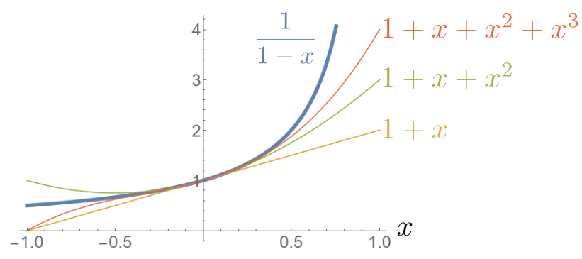
Note that it does not apply everywhere. There is a divergence at $x=1$, and convergence is slow here (meaning that even though we put a lot of terms of the Taylor expansion, we don’t approach the correct value quickly). But around $x=0$, this is excellent.
Once we know such formulae, we can obtain many more, by combinations, e.g.:
$$\frac{1}{1+x}=1-x+x^2-x^3+x^4+\cdots$$
(which is equally important). Or:
$$\frac{1}{1+x^2}=1-x^2+x^4-x^6+\cdots$$
We will conclude with this one, because it has a very beautiful result cast in it. This is plotting below, again, the exact function $1/(1+x^2)$ (in thick blue) and various terms of the Taylor expansion for increasing numbers of terms.
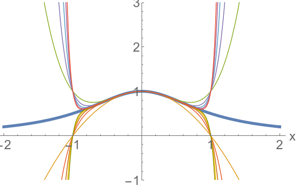
There is something shocking here. The Taylor expansion also fits very well around $x=0$, but even though we add as many terms as we want, we can’t get to approximate it beyond $x=1$ (or below $x=-1$). It’s not even that we get a poor approximation, we get a diverging series of positive and negative numbers. This is actually the same as for $1/(1-x)$ where we couldn’t get to approximate the function for $|x|>1$. In the previous case, there was a divergence so we were somehow expecting troubles there. But now, this is strange because the function itself, $1/(1+x^2)$, has no divergence. It is everywhere well defined. And smooth, and so clearly wanting for a nice approximation everywhere. But even if we’re ready to pour in as many terms as we can, even up to infinity, we can’t approximate it at, say, $x=1.5$. Why is that?
We’ll need to learn of the analysis (or calculus) of other numbers to understand this apparent mystery, namely, complex numbers. When we have complex numbers in our pocket, it will become obvious why the Taylor expansion is so constrained, even for such a nicely defined function.
But before we turn to complex analysis, we need to sharpen our Taylor approximations for common real-valued function. Using the laws that you know (or will find a way to find back and remember), please compute for yourself the Taylor series for the following, extremely important functions. And share your computations with us:
- $\sin(x)$
- $\cos(x)$
- $\tan(x)$
- $\exp(x)$
- $\ln(1+x)$
- $(1+x)^\alpha$
- $\sqrt{1+x}$ (that’s $(1+x)^{1/2}$)
- $1/\sqrt{1+x}$ (that’s $(1+x)^{-1/2}$)