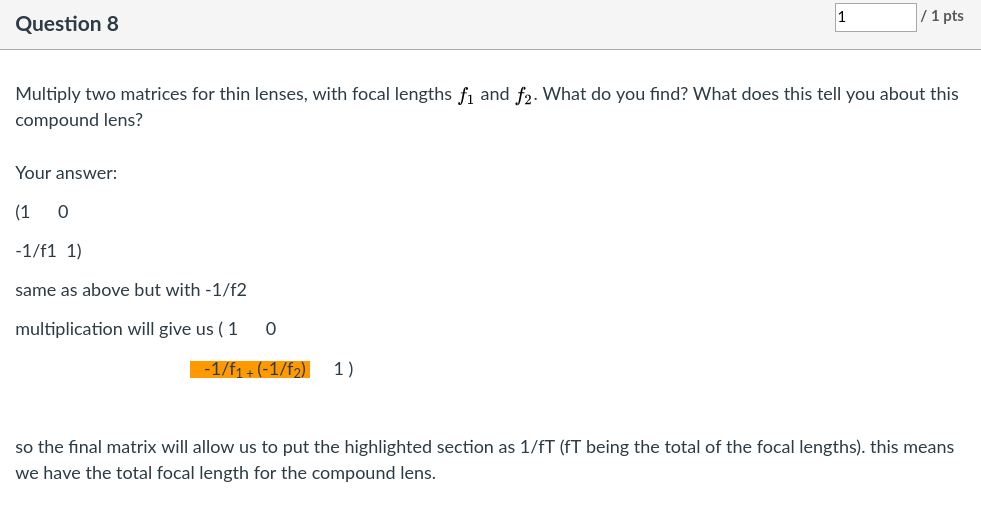
Multiply two matrices for thin lenses, with focal lengths
and
. What do you find? What does this tell you about this compound lens?
Canvas actually allows you to typeset your answer but we cover $\LaTeX$ in 2nd semester, so we have to deal with ASCII tricks, but that doesn’t matter. What does is the answer, which is here correctly given by Dilem:
I have little to add. This is another basically correct entry, with a more loose articulation of the conclusion (“focal length equal to the sum of each lens“):

These are less successful or less inspired entries:
It’s dependent on the focal length
As the focal length is here in the singular, maybe it is meant that the compound object depends on its focal length. It sounds like a tautology, or a trivial statement. It looks like the student just tried a desperate reply that sounds like the sort of answer that could grab a few points (it did get 0.25 as it’s not clearly incorrect).
They magnify
Who is “They”? The compound lens could, or not, magnify. I think this has missed the point (which was to recognize that the compound object behaves as a lens, in the first place).
(1 , -1/f2) (-1/f1, -1/f1 x -1/f2 +1) I have no idea what this tells me
Here there seems to be some error in the computation, doubled with some confusing notation. No wonder this is totally unclear what this could tell. At least the student recognizes it’s unclear rather than making a mystifying statement that would convey the impression they have a clever idea.
The matrice for a compound lense is only reliant on -1/f
Another unclear—trying-to-guess-what-answer-could-work—statement. It could be interpreted as correct, with the implication that the compound object is a lens fully determined by its focal length, which also looks a tautology, also, $f$ is not clearly defined. So unless you know the answer, I believe it’s difficult to make much sense out of this input. Quarter of a point.
And the most popular reply:
We indeed got 2 students who left this entry blank (out of those who took the Quiz in time).
This is the reasoning (adapted from our Canvas module). The matrix of a compound lens formed by putting two thin lenses back to back is given by the product of their ray matrices:
$$M_{f_1}M_{f_2}=\begin{pmatrix}1&0\\\displaystyle-\frac1f_1&1\end{pmatrix}
\begin{pmatrix}1&0\\\displaystyle-\frac1f_2&1\end{pmatrix}=\begin{pmatrix}1&0\\\displaystyle-\frac1f_1-\frac1f_2&1\end{pmatrix}$$
We can write this in a more economical but also more insightful form:
$$M_{f_1}M_{f_2}=M_{f_1f_2/(f_1+f_2)}$$
What the notation highlights is precisely the fact that the product matrix has the same form as each indivual matrix, therefore, the compound object behaves collectively as any of its single part. So two thin-lenses put back to back make another thin lens! The only obvious difference is that we now have a more involved expression for the $C$ element of the $ABCD$ matrix, but this we can always write as $-1/f_\mathrm{compound}$, and this gives us, furthemore, an expression for the compound focal length:
$$f_\mathrm{compound}=\displaystyle\frac{f_1f_2}{f_1+f_2}$$
What would have been great is an analogy to similar results familiar to the students from other fields, something like:
Focal lengths of thin lenses add like resistances put in parallel in an electric circuit.
And this observation would lead to further questions: is there a way to assemble lenses so that their focal lengths add like “in series” ($f_1+f_2$)? The fact lenses behave in this way is why we introduce the notion of vergence of optical systems. That’s maybe close to what Dylan had in mind, but he didn’t pursue it any further, I believe because of the imprecision of his formulation. A proper statement often opens natural new questions of its own, and when such a process is started, one is not merely answering a quiz on Canvas, but is doing research already…
]]>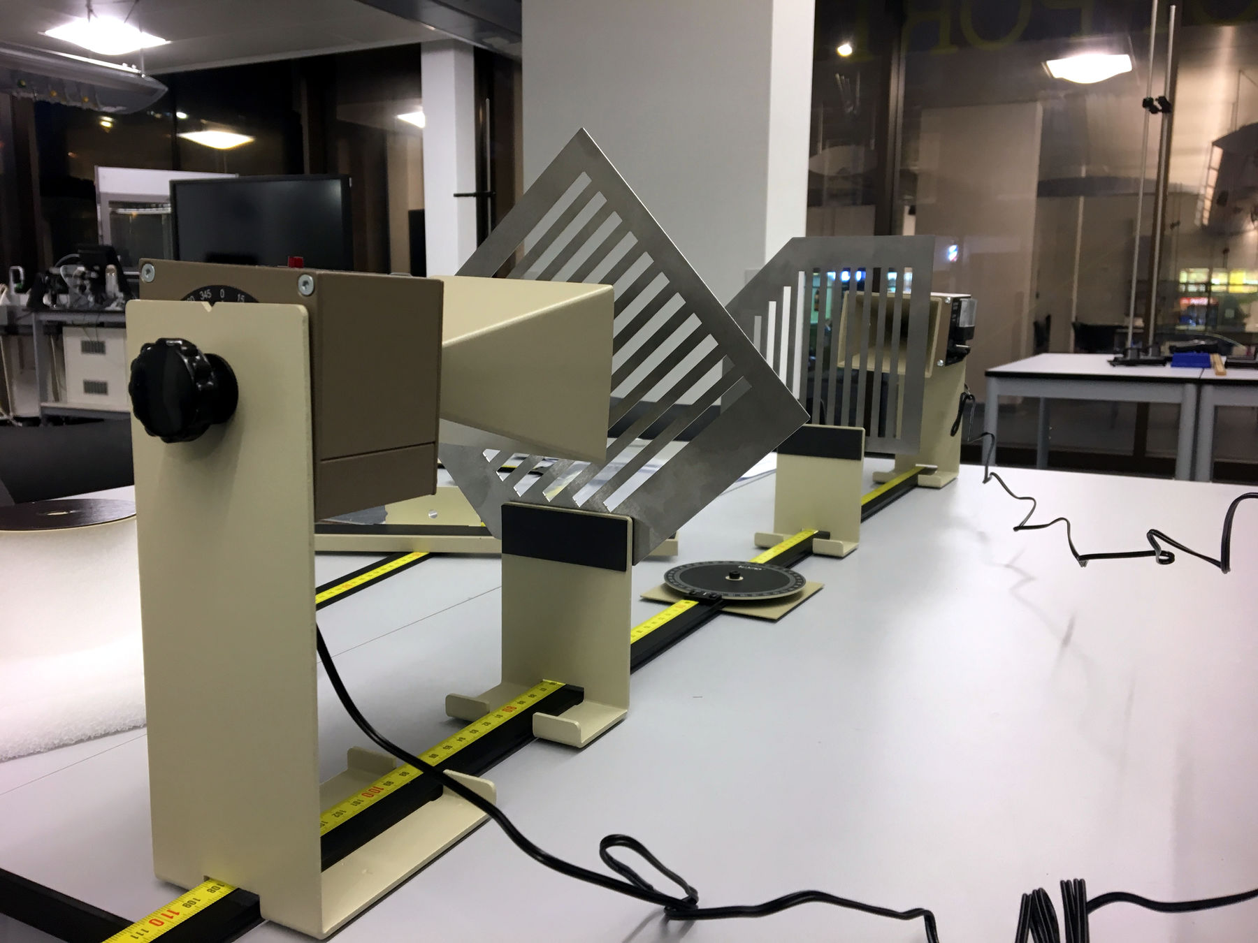
Interestingly, this is characterized as microwave optics by the provider, although these are short radiowaves. Indeed some nomenclature defines microwaves up to 10cm. Possibly because these are not useful for radio-applications, although I still find it strange to label micro something that is larger than your hand.
This is a first characterization of our setup, testing the inverse square law:
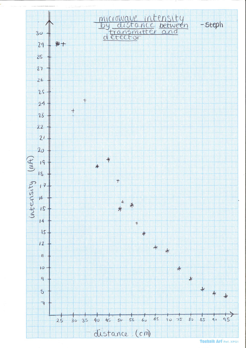
We like to plot these as $1/R^2$ to see if this follows the inverse square law, but in this case the natural variables are also interesting because, it doesn’t… there are oscillations, particularly notable at small distances (also at 70cm, it’s probably not an outlier). Here oscillations are caused by resonances and standing waves. The wavelength, I think I picked up from yesterday discussions in the lab, is 2.8cm, and more resolution is definitely called for to see the type of Physics that takes over geometry in this case, as well as possibly at larger distances where the law should be excellently satisfied (and there’s still plenty of signal at about 1m and the fall-off we have observed so far is sub-quadratic). That would require for students to tweak a bit the setup. So this is a good starting point. Maybe a nice student-research project, possibly combined with inverse square of gamma rays and light. There are great experiments we’re looking forward to do, including the double slit (of course) but also Bragg diffraction. So we’ll see much more of these things.
]]>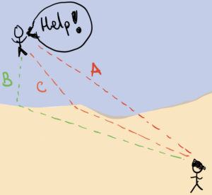 Let us consider the following scenario: on a sunny day, some people decide to go to the beach and have some fun with the waves. A coastal guard is keeping an eye on the swimmers, and she notices that one of them appears to be drowning. To help the person in distress, she has to decide which path will take her to the swimmer in the least amount of time: she could try to get to there in a straight line (path A), but in this case she would have to swim most of the way. Alternatively, she could run a lot on the sand and swim the least amount of distance (path B). However, even though humans run faster than they can swim, the most efficient way to get to the surfer is making a compromise the amount of running on the sand and swimming on the water (path C).

Light behaves in this way too. When it has to go from a point $A$ to another point $B$, it will take the path that guarantees the least amount of time, and such a path, as in the case of the coast guard, may not be a straight line. Because of this, when we put a straw in a glass of water, it looks like the straw is bending. Well, it is actually the light that is bending!
While the concept of light bending was known by the ancient Greeks, it was not until the enlightenment that the description was put in mathematical terms. Willebrord Snellius showed that the relation between the angles with which light approaches the interface in one medium and leaves the interface in the other medium are related as $$\frac{\sin \theta_1}{\sin \theta_2} = \frac{v_1}{v_2}\,,$$ where $v_1$ and $v_2$ are the velocity at which light propagates on each of the media. As nothing can travel faster than the speed of light in vacuum, it is convenient to define the velocity of propagation of light in a given medium as $v=c/n$, where $n$ is the so-called index of refraction of the medium. Thus, the relation above becomes $$\frac{\sin \theta_1}{\sin \theta_2} = \frac{n_2}{n_1}\,,$$ which is the well-known Snell’s law.
Armed with this equation, we may tackle more involved problems, as the refraction of light when the interface between the two media is spherical, as shown in the figure below.
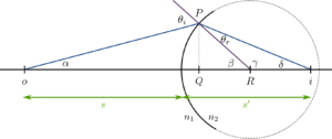
From the sketch becomes reasonable that an object placed in the medium with refraction index $n_1$ will generate an image (is it real or virtual?) on the medium with refraction index $n_2\,.$ The problem is as fundamental as it gets: we need to find the relation between the position of the object $o$, the position of the image $i$, the radius of the spherical surface $R$ and the refraction of the two media $n_1$ and $n_2$.
Let us consider a ray of light that goes from the position of the object $o$, to an arbitrary point $P$ on the spherical surface. The light impinges onto the surface at an angle $\theta_i$, as measured from the line perpendicular to the surface (shown in purple on the sketch). When passing to the medium with refraction index $n_2$, the light refracts and leaves the surface at an angle $\theta_r$ (from the sketch, does $n_2<n_1$ or $n_1<n_2$?), and continues its propagation until it reaches the optical axis.
Considering that the sum of the angles inside of a triangle is equal to $\pi$, we know that the angles in the sketch are related as follows:
- $\delta + \gamma+\theta_r=\pi$.
- $\beta+\gamma=\pi$.
- $\alpha+\beta+(\pi-\theta_i)=\pi$.
Using 1. and 2. get can get rid of the angle $\gamma$ to find $\theta_r=\beta-\delta$, and simplifying 3. we have $\theta_i = \alpha+\beta$.
Conversely, we know that
$$\tan \alpha = \frac{PQ}{oQ}\,, \quad \quad \tan \delta = \frac{PQ}{Qi} \quad \quad \mathrm{and} \quad \quad \tan \beta = \frac{PQ}{QR}\,,$$
where, for instance, $PQ$ is the distance between the points $P$ and $Q$. Furthermore, in the paraxial approximation, in which we assume that the rays are barely separated from the optical axis, we have very smalls angles an therefore: $\tan \alpha \approx \alpha$, $\tan \delta \approx \delta$, $\tan \beta \approx \beta$, $\sin \theta_i \approx \theta_i$, $\sin \theta_r \approx \theta_r$ and notably $oQ \approx s$, $Qi \approx s’$ and $QR \approx R$ . Using these approximations we have the following equations:
- From Snell’s law we have: $n_1 \theta_i = n_2 \theta_r$.
- The relation $\theta_r=\beta-\delta$ becomes $\theta_r = \frac{PQ}{R} – \frac{PQ}{s’}$.
- The relation $\theta_i = \alpha+\beta$ becomes $\theta_i = \frac{PQ}{s}+\frac{PQ}{R}$.
Joining these three equations we obtain
$$n_1 \left( \frac{PQ}{s}+\frac{PQ}{R} \right) =n_2 \left(\frac{PQ}{R} – \frac{PQ}{s’} \right)\,.$$
Dividing the two sides by the distance $PQ$ and rearranging the terms, we get
$$ \frac{n_1}{s} + \frac{n_2}{s’} = \frac{n_2-n_1}{R}\,,$$
which is the final form of our relation.
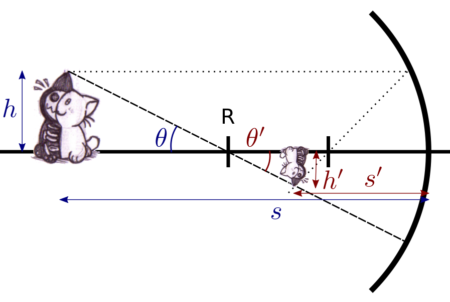
and reasoning:
The angles $\theta$ and $\theta’$ are equal as vertically opposite angles:
\begin{equation}
\label{eq:Wed10Oct162927BST2018}
\theta=\theta’
\end{equation}and they can be both related to the important quantities of the problem as follows:
\begin{align}
\tan\theta=\frac{h}{s-R}\\
\tan\theta’=\frac{h’}{s’-R}\label{eq:Wed10Oct162841BST2018}
\end{align}On the second line, I note that $h’$ is negative, which is okay as it is an algebraic quantity. Anyway, from the first equation, I can deduce that the magnification $m\equiv\displaystyle\frac{h’}{h}$ is given by
\begin{equation}
m=\frac{s’-R}{s-R}\,.
\end{equation}
However the formula which has been given in class for the magnification is:
\begin{equation}
\label{eq:Wed10Oct163138BST2018}
m=-\frac{s’}{s}\,.
\end{equation}
Can you explain to this student what is going on? (before next tutorial and/or next blog post, where an explanation will be proposed; you are welcome to share your suggestions in the comments below. If you figure it out, it should be clear what is going on).
]]>How many piano tuners are there in Chicago?
What’s your guess? Such problems became to be known as Fermi problems. By multiplying reasonable estimates (number of people in Chicago, number of people per house, percentage of households having a piano, how many times a year a piano needs tuning, how many pianos can a piano-tuner tune on a working day, etc.), one arrives at an estimate which, often, is surprisingly accurate. There is some statistics involved in the stability of such a procedure, that we will not go into today. Suffice to say that one of the most important and intriguing open questions ever posed to mankind relies on such an estimation (where is everybody? see the Drake equation).
Another useful approximation which every physicist uses is the linear approximation. This replaces an exact but awkward expression into an approximate but useful result. For instance, we have seen in the lecture on the double-slit experiment how the path difference reads straight from Pythagoras:
$$\begin{align}\Delta l&=l_2-l_1\\
&=\sqrt{(x+d/2)^2+L^2}-\sqrt{(x-d/2)^2+L^2}\tag{1}\label{eq:1}\\
&={L}\left(\sqrt{1+\left[\frac{x+d/2}{L}\right]^2}-\sqrt{1+\left[\frac{x-d/2}{L}\right]^2}\right)\\
&=\frac{xd}{L}\tag{2}\label{eq:2}\end{align}$$
and how this brings us to a useful formula—which we can keep in our collection of important results to remember—between the position of the $n$th bright fringe, at $x$, when light with wavelength $\lambda$ is projected on a screen a distance $L$ apart through a double slit of width $d$:
$$x=n\frac{\lambda L}{d}$$
The 2nd line, eq. (), is the exact result. The last line, eq. (), is the approximation when $L\gg x+d$. This is achieved by using so-called Taylor expansion, or Taylor series. Namely, we have used here the fact that:
$$\sqrt{1+\epsilon}\approx 1+\epsilon/2\tag{3}\label{eq:3}$$
which is a good approximation when $\epsilon\approx 0$. This is shown graphically below.
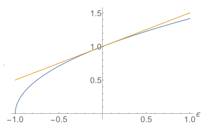
The blue line is ${\sqrt{1+\epsilon}}$ and the orange one is $1+\epsilon/2$. We have replaced a curvy shape by a line!
You can see how we approximate a complicated nonlinear function (here a square root) by a linear function. For instance, it is easy to compute that $\sqrt{1.012}$ is close to 1.006 (the real result is 1.00598, an error of less than 0.002%). It works fairly well even when $\epsilon$ is not that small. This is the percentage of relative error made:
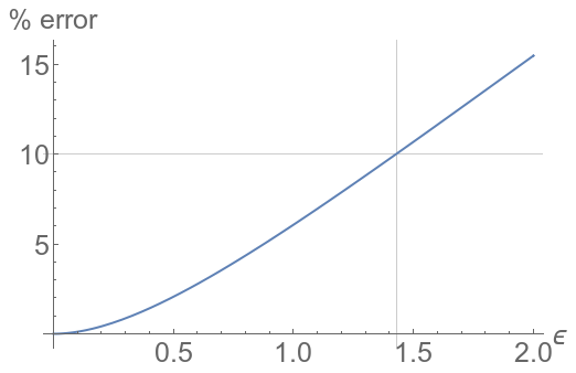
and for a qualitative understanding, 10% is acceptable. So you can happily estimate $\sqrt{1.75}$ as 1.375 (by mental calculation, we’d go first with 1.35 (1+0.7/2) and the time to say that, you could add the 0.05/2=0.025 but as this is an overestimation, as shown on the first graph, it’d be wise to stop there anyway. The real result is 1.32288, an error of about 2%).
An engineer, or a computer, would want to keep the exact result. A physicist would typically look for as much simplifications as possible (but not more). Actually, so great is the temptation that we even simplify very simple things that would not seem to require it, such as $(1+x)^2\approx 1+2x$. Here it’s from the binomial theorem. But for the general case, where does this come from anyway? At the first order, simply from the derivative, which is defined as:
$$f'(x)=\lim_{\epsilon\rightarrow0}\frac{f(x+\epsilon)-f(x)}{\epsilon}$$
That’s the definition of a Mathematician. For us, it becomes:
$$f'(x)\approx\frac{f(x+\epsilon)-f(x)}{\epsilon}$$
The limit means that it becomes exact when $\epsilon$ is vanishing. For any finite value, this is only an approximation (a better one the smaller the $\epsilon$, but an approximation nonetheless). For us who, like in the army, are still happy with a 10% loss, the limit can just be overlooked. Rearranging, we get:
$$f(x+\epsilon)\approx f(x)+\epsilon f'(x)$$
If we take $f=\sqrt{}$, $x=1$ and $\epsilon$ a small number, remembering that $\sqrt{x}’=1/(2\sqrt{x})$, we arrive at the result above, eq. (). Two things are now in order:
- We need to know this trick for all the recurring nonlinear functions we will meet (and we’ll meet a lot of them!)
- Sometimes the 1st order is not enough, so it’d be good to have approximations beyond this.
This can be done thanks to the complete Taylor formula, which you will demonstrate in your Math course:
$$f(x+\epsilon)=\sum_{n=0}^\infty\frac{f^{(n)}(x)}{n!}\epsilon$$
This is an exact (Mathematical) result… although there’s no limit! it’s because we’re summing up to infinity. $f^{(n)}$ stands for the $n$th derivative. So this becomes, back to approximating (we don’t really have time for the infinite):
$$f(x+\epsilon)\approx f(x)+f'(x)\epsilon+f^{\prime\prime}(x)\frac{\epsilon^2}{2}+f^{\prime\prime\prime}(x)\frac{\epsilon^3}{6}+f^{\prime\prime\prime\prime}(x)\frac{\epsilon^4}{24}+\cdots$$
(you remember that n! is n-factorial, right?) Here we have a fourth-order expansion (and leaving open for more). The Taylor formula is also usefully (and probably more commonly) encountered in this (equivalent) form:
$$f(x)=\sum_{k=0}^\infty f^{(n)}(a)\frac{(x-a)}{n!}=f(a)+f'(a)(x-a)+f^{\prime\prime}(a)\frac{(x-a)^2}{2}+\cdots$$
Here’s an example with another important (and recurrent) nonlinear function: the inverse. This gives the geometric series $\sum x^k$:
$$\frac{1}{1-x}=1+x+x^2+x^3+\cdots$$
And this is the graphical representation.
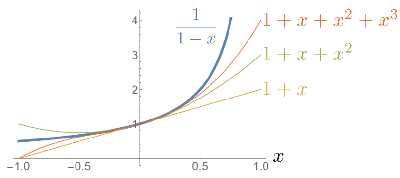
Note that it does not apply everywhere. There is a divergence at $x=1$, and convergence is slow here (meaning that even though we put a lot of terms of the Taylor expansion, we don’t approach the correct value quickly). But around $x=0$, this is excellent.
Once we know such formulae, we can obtain many more, by combinations, e.g.:
$$\frac{1}{1+x}=1-x+x^2-x^3+x^4+\cdots$$
(which is equally important). Or:
$$\frac{1}{1+x^2}=1-x^2+x^4-x^6+\cdots$$
We will conclude with this one, because it has a very beautiful result cast in it. This is plotting below, again, the exact function $1/(1+x^2)$ (in thick blue) and various terms of the Taylor expansion for increasing numbers of terms.
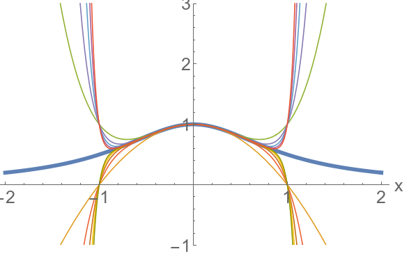
There is something shocking here. The Taylor expansion also fits very well around $x=0$, but even though we add as many terms as we want, we can’t get to approximate it beyond $x=1$ (or below $x=-1$). It’s not even that we get a poor approximation, we get a diverging series of positive and negative numbers. This is actually the same as for $1/(1-x)$ where we couldn’t get to approximate the function for $|x|>1$. In the previous case, there was a divergence so we were somehow expecting troubles there. But now, this is strange because the function itself, $1/(1+x^2)$, has no divergence. It is everywhere well defined. And smooth, and so clearly wanting for a nice approximation everywhere. But even if we’re ready to pour in as many terms as we can, even up to infinity, we can’t approximate it at, say, $x=1.5$. Why is that?
We’ll need to learn of the analysis (or calculus) of other numbers to understand this apparent mystery, namely, complex numbers. When we have complex numbers in our pocket, it will become obvious why the Taylor expansion is so constrained, even for such a nicely defined function.
But before we turn to complex analysis, we need to sharpen our Taylor approximations for common real-valued function. Using the laws that you know (or will find a way to find back and remember), please compute for yourself the Taylor series for the following, extremely important functions. And share your computations with us:
- $\sin(x)$
- $\cos(x)$
- $\tan(x)$
- $\exp(x)$
- $\ln(1+x)$
- $(1+x)^\alpha$
- $\sqrt{1+x}$ (that’s $(1+x)^{1/2}$)
- $1/\sqrt{1+x}$ (that’s $(1+x)^{-1/2}$)