Interestingly, this is characterized as microwave optics by the provider, although these are short radiowaves. Indeed some nomenclature defines microwaves up to 10cm. Possibly because these are not useful for radio-applications, although I still find it strange to label micro something that is larger than your hand.

This is a first characterization of our setup, testing the inverse square law:

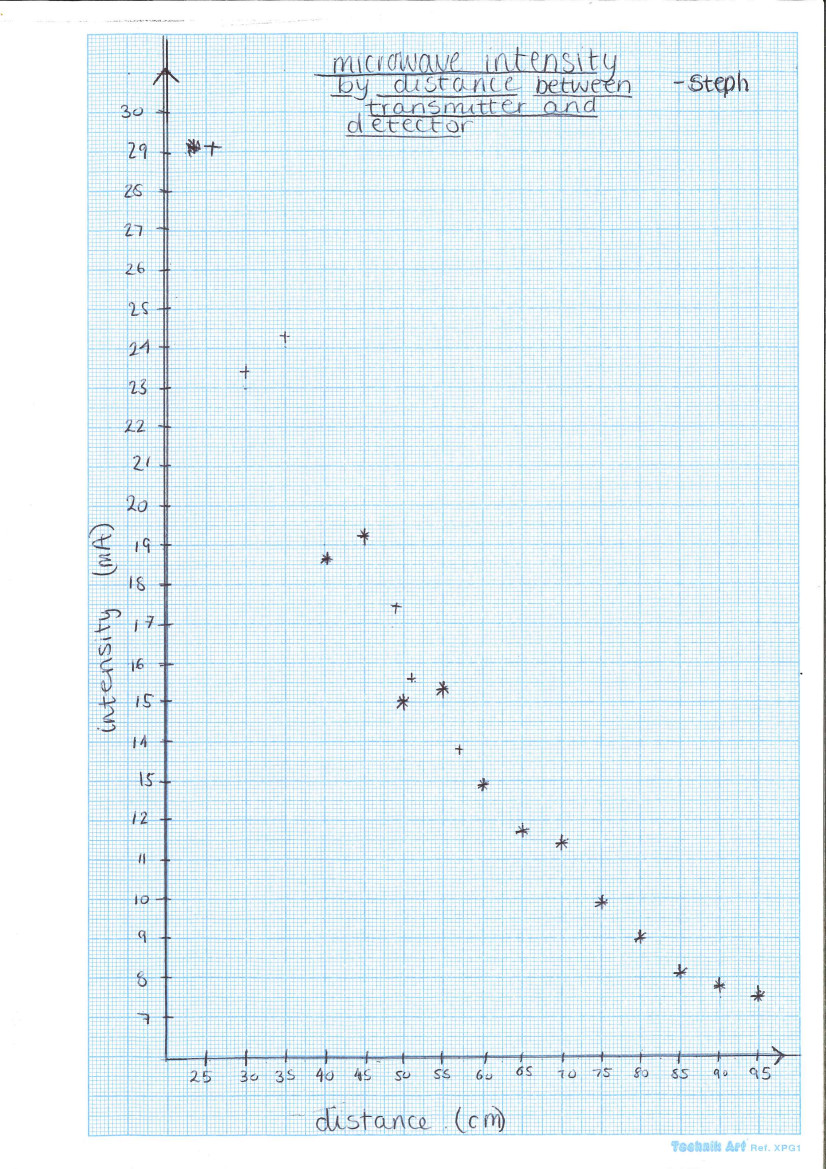
We like to plot these as $1/R^2$ to see if this follows the inverse square law, but in this case the natural variables are also interesting because, it doesn’t… there are oscillations, particularly notable at small distances (also at 70cm, it’s probably not an outlier). Here oscillations are caused by resonances and standing waves. The wavelength, I think I picked up from yesterday discussions in the lab, is 2.8cm, and more resolution is definitely called for to see the type of Physics that takes over geometry in this case, as well as possibly at larger distances where the law should be excellently satisfied (and there’s still plenty of signal at about 1m and the fall-off we have observed so far is sub-quadratic). That would require for students to tweak a bit the setup. So this is a good starting point.  Maybe a nice student-research project, possibly combined with inverse square of gamma rays and light. There are great experiments we’re looking forward to do, including the double slit (of course) but also Bragg diffraction. So we’ll see much more of these things.

How many piano tuners are there in Chicago?

What’s your guess? Such problems became to be known as Fermi problems. By multiplying reasonable estimates (number of people in Chicago, number of people per house, percentage of households having a piano, how many times a year a piano needs tuning, how many pianos can a piano-tuner tune on a working day, etc.), one arrives at an estimate which, often, is surprisingly accurate. There is some statistics involved in the stability of such a procedure, that we will not go into today. Suffice to say that one of the most important and intriguing open questions ever posed to mankind relies on such an estimation (where is everybody? see the Drake equation).

Another useful approximation which every physicist uses is the linear approximation. This replaces an exact but awkward expression into an approximate but useful result. For instance, we have seen in the lecture on the double-slit experiment how the path difference reads straight from Pythagoras:

$$\begin{align}\Delta l&=l_2-l_1\\
&=\sqrt{(x+d/2)^2+L^2}-\sqrt{(x-d/2)^2+L^2}\tag{1}\label{eq:1}\\
&={L}\left(\sqrt{1+\left[\frac{x+d/2}{L}\right]^2}-\sqrt{1+\left[\frac{x-d/2}{L}\right]^2}\right)\\
&=\frac{xd}{L}\tag{2}\label{eq:2}\end{align}$$

and how this brings us to a useful formula—which we can keep in our collection of important results to remember—between the position of the $n$th bright fringe, at $x$, when light with wavelength $\lambda$ is projected on a screen a distance $L$ apart through a double slit of width $d$:

$$x=n\frac{\lambda L}{d}$$

The 2nd line, eq. ($\text{1}$), is the exact result. The last line, eq. ($\text{2}$), is the approximation when $L\gg x+d$. This is achieved by using so-called Taylor expansion, or Taylor series. Namely, we have used here the fact that:

$$\sqrt{1+\epsilon}\approx 1+\epsilon/2\tag{3}\label{eq:3}$$

which is a good approximation when $\epsilon\approx 0$. This is shown graphically below.

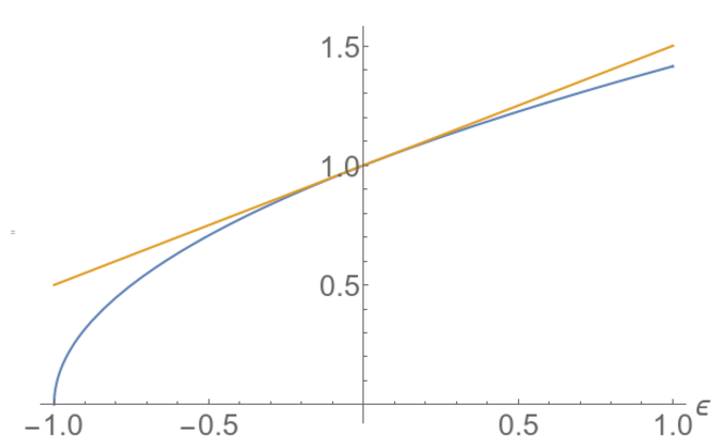
The blue line is ${\sqrt{1+\epsilon}}$ and the orange one is $1+\epsilon/2$. We have replaced a curvy shape by a line!

You can see how we approximate a complicated nonlinear function (here a square root) by a linear function. For instance, it is easy to compute that $\sqrt{1.012}$ is close to 1.006 (the real result is 1.00598, an error of less than 0.002%). It works fairly well even when $\epsilon$ is not that small. This is the percentage of relative error made:

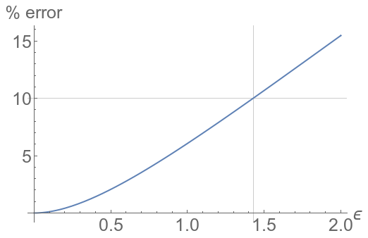
and for a qualitative understanding, 10% is acceptable. So you can happily estimate $\sqrt{1.75}$ as 1.375 (by mental calculation, we’d go first with 1.35 (1+0.7/2) and the time to say that, you could add the 0.05/2=0.025 but as this is an overestimation, as shown on the first graph, it’d be wise to stop there anyway. The real result is 1.32288, an error of about 2%).

An engineer, or a computer, would want to keep the exact result. A physicist would typically look for as much simplifications as possible (but not more). Actually, so great is the temptation that we even simplify very simple things that would not seem to require it, such as $(1+x)^2\approx 1+2x$. Here it’s from the binomial theorem. But for the general case, where does this come from anyway? At the first order, simply from the derivative, which is defined as:

$$f'(x)=\lim_{\epsilon\rightarrow0}\frac{f(x+\epsilon)-f(x)}{\epsilon}$$

That’s the definition of a Mathematician. For us, it becomes:

$$f'(x)\approx\frac{f(x+\epsilon)-f(x)}{\epsilon}$$

The limit means that it becomes exact when $\epsilon$ is vanishing. For any finite value, this is only an approximation (a better one the smaller the $\epsilon$, but an approximation nonetheless). For us who, like in the army, are still happy with a 10% loss, the limit can just be overlooked. Rearranging, we get:
$$f(x+\epsilon)\approx f(x)+\epsilon f'(x)$$
If we take $f=\sqrt{}$, $x=1$ and $\epsilon$ a small number, remembering that $\sqrt{x}’=1/(2\sqrt{x})$, we arrive at the result above, eq. ($\text{3}$). Two things are now in order:

1. We need to know this trick for all the recurring nonlinear functions we will meet (and we’ll meet a lot of them!)
2. Sometimes the 1st order is not enough, so it’d be good to have approximations beyond this.

This can be done thanks to the complete Taylor formula, which you will demonstrate in your Math course:

$$f(x+\epsilon)=\sum_{n=0}^\infty\frac{f^{(n)}(x)}{n!}\epsilon$$

This is an exact (Mathematical) result… although there’s no limit! it’s because we’re summing up to infinity. $f^{(n)}$ stands for the $n$th derivative. So this becomes, back to approximating (we don’t really have time for the infinite):

$$f(x+\epsilon)\approx f(x)+f'(x)\epsilon+f^{\prime\prime}(x)\frac{\epsilon^2}{2}+f^{\prime\prime\prime}(x)\frac{\epsilon^3}{6}+f^{\prime\prime\prime\prime}(x)\frac{\epsilon^4}{24}+\cdots$$

(you remember that n! is n-factorial, right?) Here we have a fourth-order expansion (and leaving open for more). The Taylor formula is also usefully (and probably more commonly) encountered in this (equivalent) form:

$$f(x)=\sum_{k=0}^\infty f^{(n)}(a)\frac{(x-a)}{n!}=f(a)+f'(a)(x-a)+f^{\prime\prime}(a)\frac{(x-a)^2}{2}+\cdots$$

Here’s an example with another important (and recurrent) nonlinear function: the inverse. This gives the geometric series $\sum x^k$:

$$\frac{1}{1-x}=1+x+x^2+x^3+\cdots$$

And this is the graphical representation.

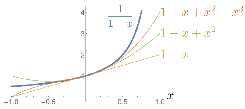
Note that it does not apply everywhere. There is a divergence at $x=1$, and convergence is slow here (meaning that even though we put a lot of terms of the Taylor expansion, we don’t approach the correct value quickly). But around $x=0$, this is excellent.

Once we know such formulae, we can obtain many more, by combinations, e.g.:

$$\frac{1}{1+x}=1-x+x^2-x^3+x^4+\cdots$$

(which is equally important). Or:

$$\frac{1}{1+x^2}=1-x^2+x^4-x^6+\cdots$$

We will conclude with this one, because it has a very beautiful result cast in it. This is plotting below, again, the exact function $1/(1+x^2)$ (in thick blue) and various terms of the Taylor expansion for increasing numbers of terms.

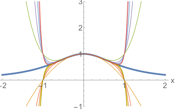
There is something shocking here. The Taylor expansion also fits very well around $x=0$, but even though we add as many terms as we want, we can’t get to approximate it beyond $x=1$ (or below $x=-1$). It’s not even that we get a poor approximation, we get a diverging series of positive and negative numbers. This is actually the same as for $1/(1-x)$ where we couldn’t get to approximate the function for $|x|>1$. In the previous case, there was a divergence so we were somehow expecting troubles there. But now, this is strange because the function itself, $1/(1+x^2)$, has no divergence. It is everywhere well defined. And smooth, and so clearly wanting for a nice approximation everywhere. But even if we’re ready to pour in as many terms as we can, even up to infinity, we can’t approximate it at, say, $x=1.5$. Why is that?

We’ll need to learn of the analysis (or calculus) of other numbers to understand this apparent mystery, namely, complex numbers. When we have complex numbers in our pocket, it will become obvious why the Taylor expansion is so constrained, even for such a nicely defined function.

But before we turn to complex analysis, we need to sharpen our Taylor approximations for common real-valued function. Using the laws that you know (or will find a way to find back and remember), please compute for yourself the Taylor series for the following, extremely important functions. And share your computations with us:

• $\sin(x)$
• $\cos(x)$
• $\tan(x)$
• $\exp(x)$
• $\ln(1+x)$
• $(1+x)^\alpha$
• $\sqrt{1+x}$ (that’s $(1+x)^{1/2}$)
• $1/\sqrt{1+x}$ (that’s $(1+x)^{-1/2}$)

The square of the orbital period of a planet is proportional to the cube of the semi-major axis of its orbit.

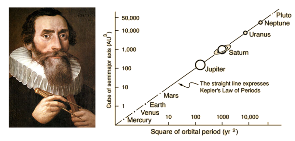
This resulted from many observations and a lot of fiddling with numbers (allegedly stolen from Tycho Brahe), until this mysterious relationship was discovered, a feast which impressed Einstein himself. The delight of the discovery was penned by the author of the harmonies of the world in a way unfortunately not available nowadays to scientific publications:

I first believed I was dreaming… But it is absolutely certain and exact that the ratio which exists between the period times of any two planets is precisely the ratio of the 3/2th power of the mean distance.

It was a bit strange and as most people who come with something genuinely new, poor Kepler met with much criticism. His own mentor (some now-forgotten Michael Mästlin) objected to him that “One should only treat astronomical things astronomically and not mix them with earthly physics.” The greatest breakthrough in Physics, Newton’s Universal theory of gravitation, would precisely show that Physics is what mixes earthly things like falling apples with astronomical ones like the falling moon.

We used this example during induction week as an illustration of the difference between an empirical law (Johannes’ observation cooked up into three particular laws) and a theoretical model (Newton’s theory expressed into three general and far-reaching laws). Another example we discussed is Rydberg’s formula and Bohr model of the atom, to explain the spectral lines of hydrogen.

How Newton derived Kepler’s law is a topic in Mechanics. Two of our students already knew the trick, and could reconstruct it… during the lecture! This is the note handed over by Luke after the class:

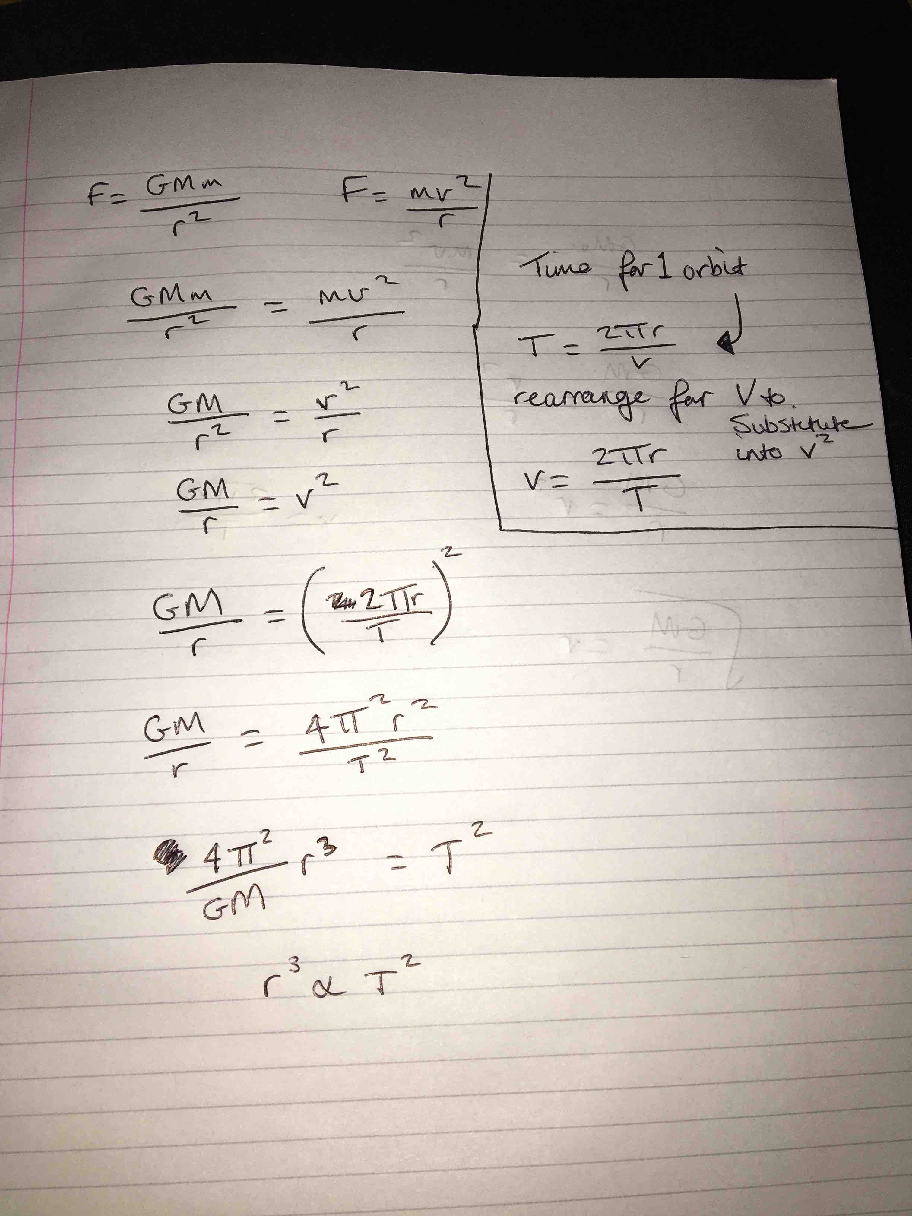
Well done! And came another, more detailed derivation from Joel, which went along the same line. To have something new to show, we asked Joel to compute the numerical value of Kepler’s constant in SI units (which we also covered) and this is what he found

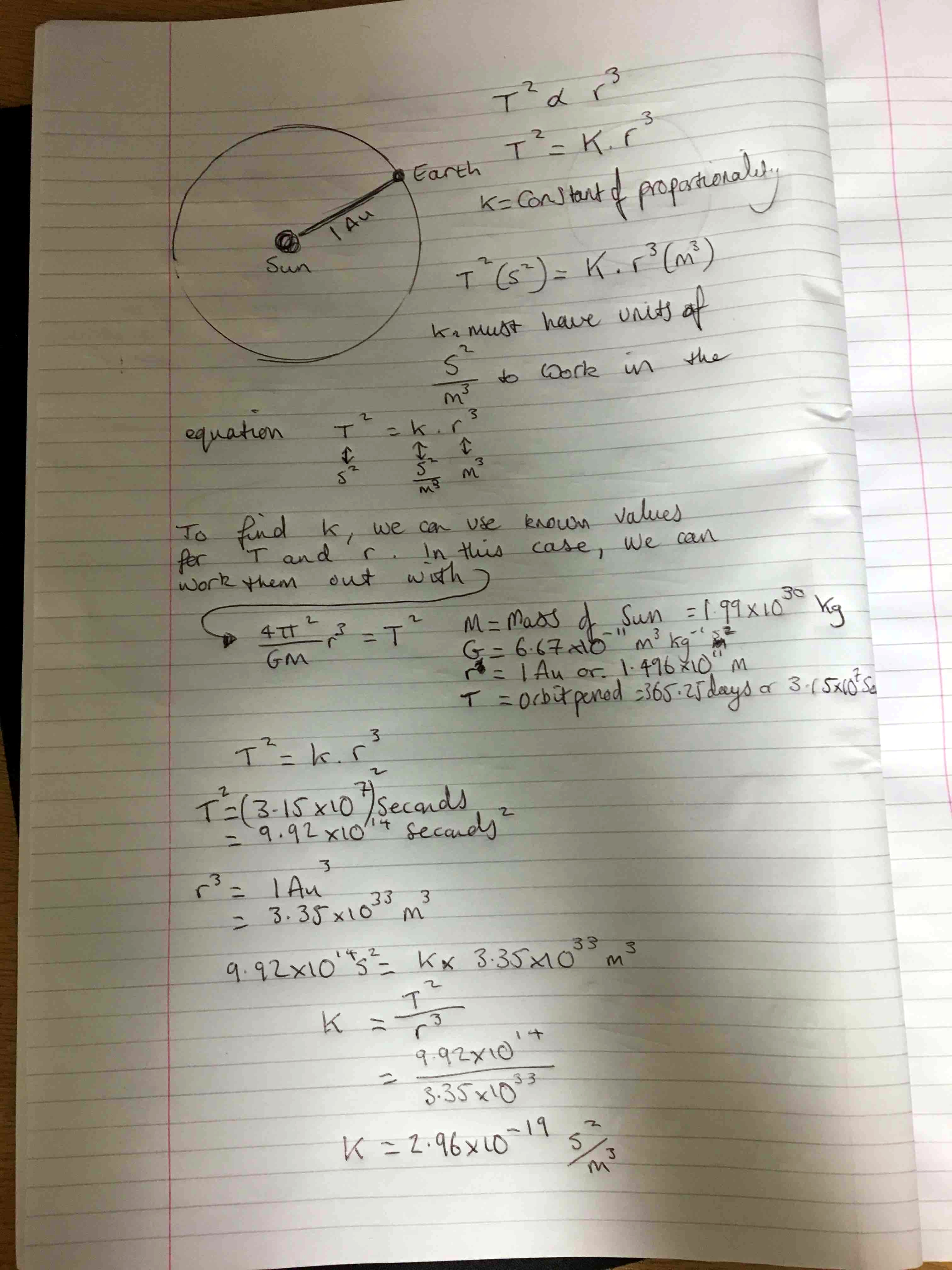
That is, 7.52 MAU$^3$/day$^2$ (MAU is Mega-Astronomical units), vs 7.51 for Kepler’s average over six planets. These are the units from the Wikipedia (as also used by Kepler). They should really be in Mau$^3$/year$^2$ in which case the number is much more meaningful in itself (and is not exactly 1 for Earth, do you see why? We have a comment section if you want to contribute your thoughts).

Planetary motion will definitely make several comebacks in our Mechanics course, taught by an astro-solar-mathematico-physicist, and so will Rydberg’s formula, although it is not until the end of Year 5 that the connection will be established in this case (and so far we did not receive any back-of-the-envelope derivation for that). It’s also my birthday today, so I’ll leave the connection between empirical observations and theoretical models at that for today.