One of our favourite outreach setups is the magnetic pipe experiment: two pellets fall at the same rate in vacuum, but pass them through a pipe and one of the two takes ages to get through. If you peep in, you’ll see it being mysteriously slowed down without touching anything. What is going on?
One is a magnet. Although the pipe itself is not magnetic (the effect would otherwise be quite easy to understand), there is some sort of magnetic interaction. This is a manifestation of magnetic braking, itself a direct consequence of Maxwell’s equations as they turn into Faraday’s and Lenz’s laws. Faraday’s law tells you that a changing magnetic field creates an electric field. It is really the Maxwell-Faraday equation that tells you that:
$${\displaystyle \nabla \times \mathbf {E} =-{\frac {\partial \mathbf {B} }{\partial t}}}$$
where ${\frac {\partial \mathbf {B} }{\partial t}}$ means that the magnetic field $\mathbf{B}$ is changing and this causes a curl (or rotation) of the electric field $\mathbf{E}$.
If there is a conductor nearby, the electric field will set charges in motions, creating a current, and that is really where Faraday’s law gets on stage: it tells you the force of the so-called electromotive force that pushes the electrons in the conductor as a result of the changing $\mathbf{B}$. Now another of the Maxwell’s equations, that named after Ampère, says that an electric current $\mathbf{F}$ creates a magnetic field (and also that a changing electric field creates a magnetic field, because everything’s changing I give you the full equation: ${\nabla \times \mathbf {B} =\mu _{0}\left(\mathbf {J} +\varepsilon _{0}{\frac {\partial \mathbf {E} }{\partial t}}\right)}$). Lenz’s law tells us, basically, that the magnetic field created by the current itself created by the changing magnetic field opposes the change, that is, if the external magnetic field grows, the generated current will create an opposite magnetic field to keep it small, if the external magnetic field shrinks, the generated current will create an opposite magnetic field to keep it big. That comes as a minus sign in the equation that relates the electromotive force $\mathcal {E}$ and the change of the change (${d\over dt}$) of the magnetic flux $\int_\mathrm{Area}\mathbf {B} \cdot d\mathbf{S}$ (which is how the change of the magnetic field is to be tracked):
$$\displaystyle {\mathcal {E}}=-{d\over dt}\int_\mathrm{Area}\mathbf {B} \cdot d\mathbf{S}$$
It’s a lot of stuff for something so simple as a magnet falling through a pipe. There is something generated dynamically, which causes a back-reaction, leading to some equilibrium. Beautiful Physics. That deserves to be studied in details. So far, we only use it as a striking (and mysterious, if you have not heard of it before) demo with only the gist of the explanation. At some point, we will put a couple of students to study this in details as part of their Electromagnetism project. But our first quantitative study started on the occasion of a visit from our neighbours from the Oldbury wells school, who spent a morning with us along with their Physics teacher Mal (whom we meet at our IOP meetings) and with whom we discussed various aspects of free fall last Thursday. Regarding this particular experiment, we asked them to work out the velocity of the magnetic pellet inside the pipe. In however way they see fit.
What they did is best recorded through the recollection of one of the students, Annabel. She writes:
This is the picture of the results recorded:
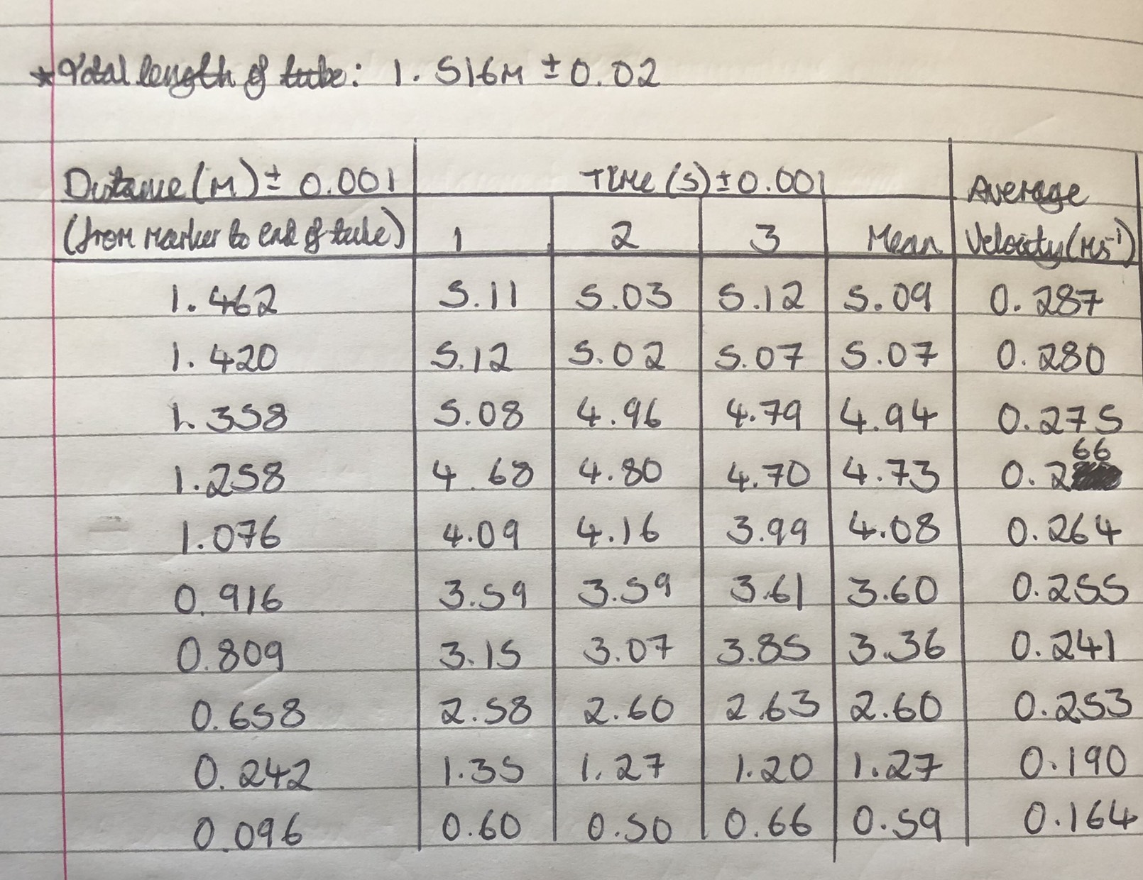
Neat and tidy. Even collecting several points for each measurement (we didn’t ask for that). But in this form, the results turn out to be very difficult to interpretate. Annabel and friends carried on to obtain the distance the magnet fell (from the mark to the end of the tube) and the average time taken for the magnet to fall this distance, from which they got average velocities for each distance. These are the results:
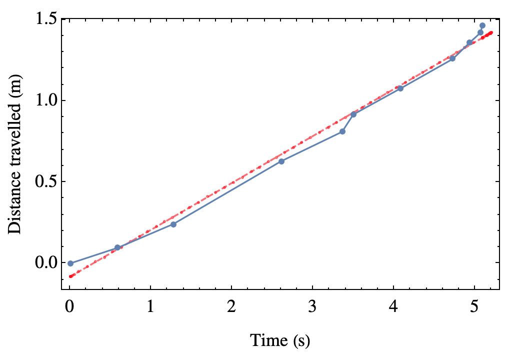
That gives an average speed of 0.288 m/s. Even working out the correct theory, we found it difficult to draw any conclusions on the terminal velocity from the experiment made in this way.
Therefore, we gave it another shot, this time in a more natural configuration of measuring from the top of the tube, rather than from the bottom. This was carefully done by our skilled assistant, Kasia, who got the following results for the same “observable” as above:
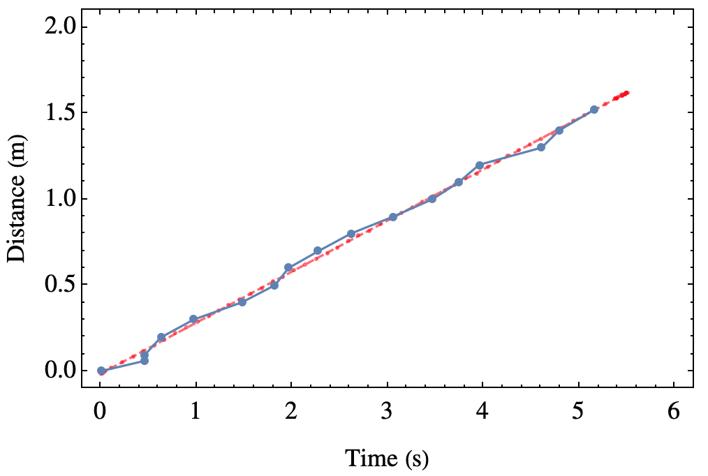
This is in agreement with the other measurement made in fairly different configuration. The average velocity in this case is 0.297 m/s. Now it escapes my memory if Kasia (and Gregor, she came with her own assistant on this occasion) also took error bars, that we ignored anyway, but it seems the two approaches are compatible. This approach, however, allows to measure the instantaneous speed, and gives clear and strong results on the terminal velocity:
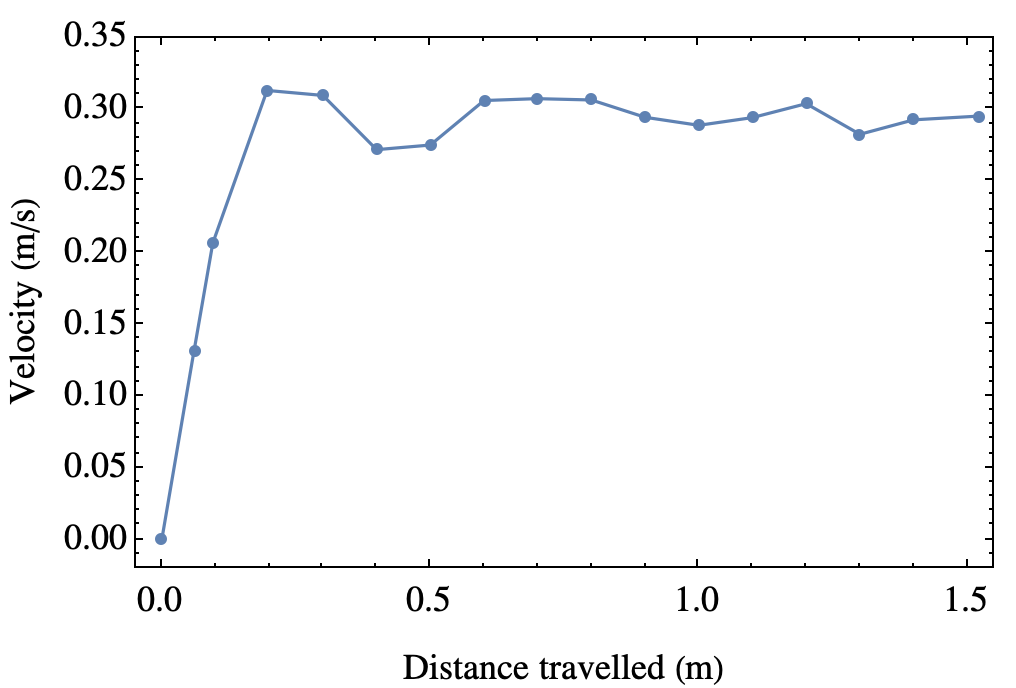
It is around 0.29m/s indeed, but here, you also see that it is a terminal velocity (a plateau) and you can see how quickly it is reached. Beautiful. In this graph it’d be worth putting error bars, but this starts to look like a B.Sc semester project rather than a short session to get a grip of free-falling objects.
If you look at the literature, there are many interesting attempts at describing the terminal velocity of a falling magnet. Maybe the best description one can find is that of Levin et al. in the American Journal of Physics 74, 815 (2006) (also available freely on the arXiv). This link points us to a formula derived in Zangwill’s Modern Electrodynamics. In this other work, people built a device with two Hall-effect switches to directly measure the terminal velocity (as a function of the thickness of their pipe, following a more detailed theoretical model of Donoso et al. in Eur. J. Phys. 30 855). Someone else provides numerical simulations of the fields. This recent work has a great bibliography. Etc., etc, there is a lot of material available. This blog post is only our first attempt at contributing something into this direction. We will provide a closer look at both the theoretical and experimental aspects of this spectacular effect. Maybe even the young people of Oldburywells will be the one telling us the rest of the story would they come back and give this problem more thoughts and re-iterated efforst (as part of a University-student career, maybe).